Optimizing Solar Power Collection for StratoSonde

Optimizing Solar Power Collection for StratoSonde

Solar power is the lifeblood of long-duration stratospheric balloon missions, but extracting maximum energy from small panels requires more than plugging in a datasheet value. For Stratosonde, I needed to answer three critical questions: How much power can we actually harvest? What’s the optimal panel orientation for a free-spinning payload? And how do we configure the power management IC to capture every available milliwatt?

The answers came from systematic I-V curve measurements, cosine loss calculations, and global performance modeling. This post documents the characterization of Aoshike 52x19mm polycrystalline silicon cells (0.5V nominal) and the engineering decisions that followed—from horizontal mounting rationale to precise MPPT ratio tuning for the BQ25570 energy harvester.

Beyond Basic Specs

Open-circuit voltage (Voc) and short-circuit current (Isc) validate the datasheet, but they don’t tell you how much usable power reaches the boost converter. To find the Maximum Power Point (MPP), I swept a resistive load across the panel while measuring voltage and current, generating I–V curves and power–voltage curves to see exactly where V×I peaks.

That MPP is what the BQ25570 energy-harvesting IC has to lock onto. Configure it wrong and a big chunk of available power never makes it into the batteries.

Characterization Results

I collected I–V curves under four scenarios in Calgary (November, 51°N latitude):

• 10:00 AM, sun-tracking: panel perpendicular to the sun
• 12:00 PM, sun-tracking: peak solar elevation
• 12:30 PM, horizontal: panel flat, as it would fly
• 12:30 PM, 20° off-axis: simulating misalignment / self-shadowing

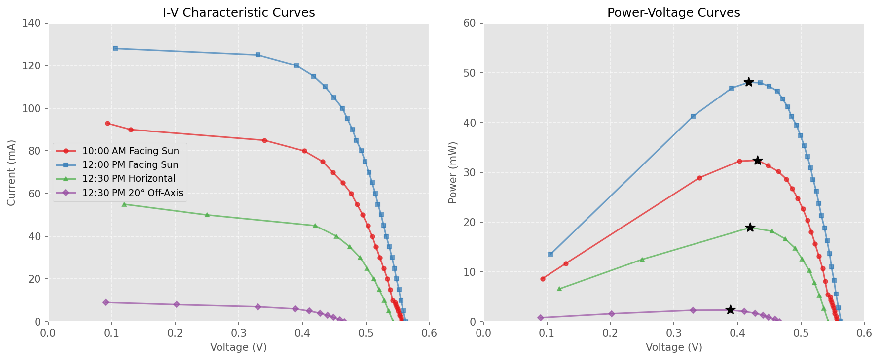
At noon, peak power rose from ~18 mW (horizontal) to ~48 mW (sun-tracking), about a 2.7× increase. The 20° test was particularly revealing: at Calgary’s low sun angle, the panel self-shadowed part of the cell, knocking output down much more than the cosine loss alone would suggest—plummeting to just 2.3 mW.

Why Horizontal Mounting

So if sun-tracking gives 2–3× more instantaneous power, why mount the panel horizontally?

The answer involves both the limitations of balloon-borne payloads and the trade-offs across different operating latitudes.

The Azimuth Problem: The balloon spins unpredictably around a roughly vertical axis with no attitude control. A vertical panel would face away from the sun roughly half the time, averaging near zero. A horizontal panel always presents the same projected area to the sun regardless of spin direction.

The Latitude Problem: Horizontal mounting is inherently latitude-dependent. At high latitudes (like Calgary at 51°N in November), the sun’s maximum elevation is only ~15-20° above the horizon at solar noon.

Let’s calculate the cosine loss explicitly. When sunlight hits a surface at an angle, the effective power per unit area scales as the cosine of the incident angle (the angle between the sun ray and the surface normal):

[ P_{\text{effective}} = P_{\text{incident}} \times \cos(\theta) ]

For a horizontal panel at Calgary in November:

• Sun elevation: ~17° above horizon
• Incident angle θ = 90° - 17° = 73° from panel normal
• Cosine loss: (\cos(73°) \approx 0.29) → 29% of perpendicular power

This is why the horizontal panel measured only 18.9 mW compared to 48.1 mW sun-tracking—it’s not just cosine loss (which predicts 29%), but also frame shadowing and oblique angle effects that drive it even lower.

Now, could we tilt the panel to improve this? In Calgary’s case: if we tilted 20° from horizontal, but the sun is only at 17° elevation, the panel would be tilted past the sun—actually receiving even less direct light. To intercept the sun perpendicularly at noon, we’d need to tilt ~73° from horizontal (nearly vertical), which creates the azimuth problem: without rotation control, this near-vertical panel faces away from the sun half the time, averaging near zero power.

The Pragmatic Choice: For a global stratospheric platform that may launch from mid-latitudes but drift toward the tropics (or vice versa):

• Horizontal mounting provides consistent, predictable performance regardless of latitude or payload rotation
• Adding tilt mechanisms increases complexity, weight, and failure modes

But what about seasonal and latitude variation? To visualize how solar power varies across the entire globe throughout the year:

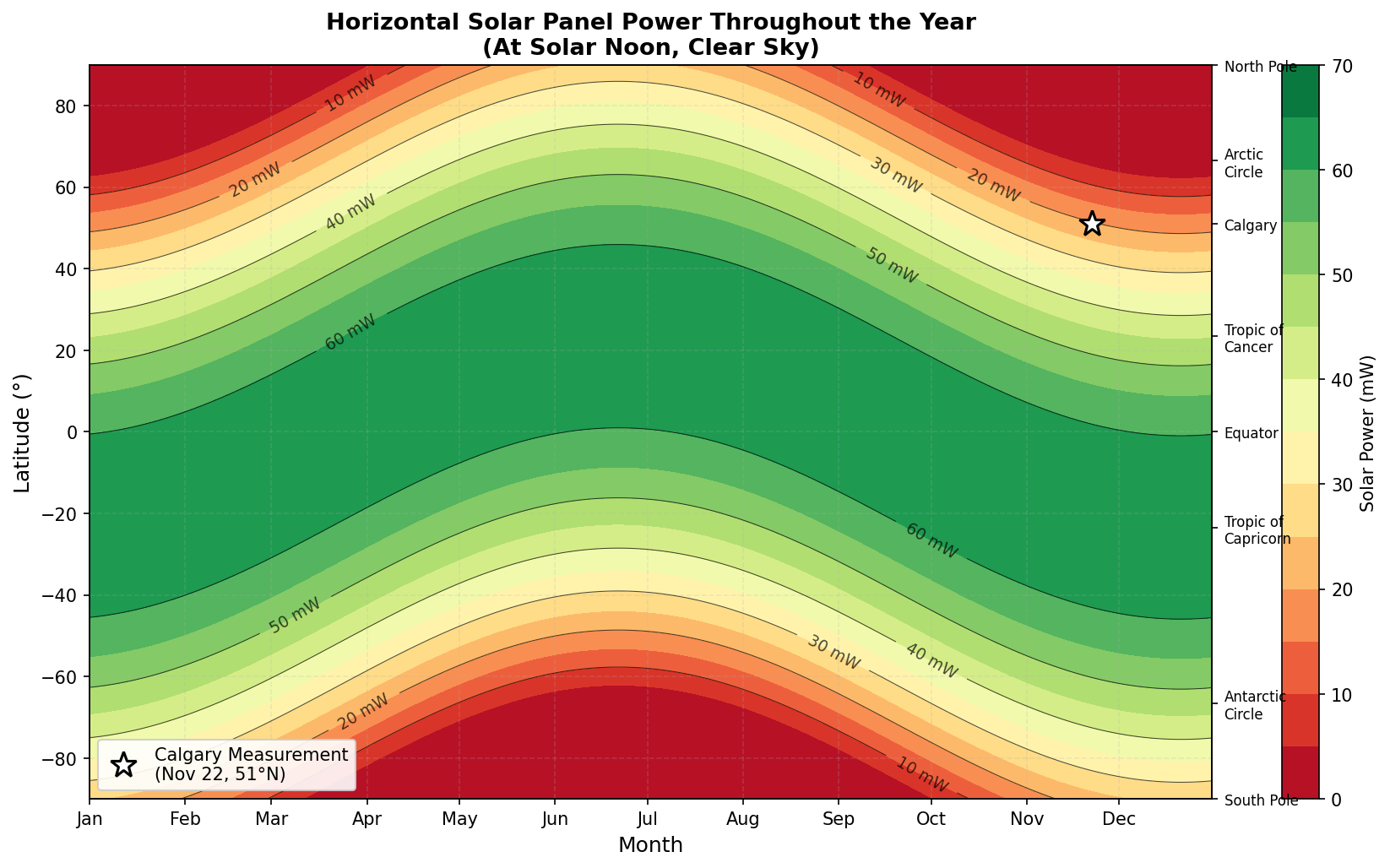
This heatmap shows the expected horizontal panel power at solar noon across all latitudes and seasons for a single 52x19mm solar cell. Key observations:

• Equator: Consistently high power year-round (~60 mW), with minimal seasonal variation
• Mid-latitudes (30-50°N): Strong summer performance (50-60 mW) but dramatic winter drop
• Calgary (51°N): Peaks at ~58 mW in June, drops to ~17 mW in December—more than 3× variation
• Arctic regions (>66°N): Reasonable summer power (~48 mW at solstice) but essentially zero in winter

The measurement point (white star) sits in the dark green “marginal power” zone, confirming that late November at 51°N represents one of the most challenging operational scenarios for horizontal solar panels.

Configuring the Power System

The TI BQ25570 energy harvesting IC uses a “fractional Open Circuit Voltage” (Voc) method to estimate the Maximum Power Point. Instead of actively tracking the peak (which requires complex, power-hungry logic), it periodically samples Voc and regulates the input voltage to a fixed percentage of that sampled value. This percentage is set by the ratio of external resistors (ROC1/ROC2).

Looking at our data:

• Voc (Open Circuit Voltage): Approximately 0.56 V in direct sun.
• Vmpp (Maximum Power Voltage): Approximately 0.42 V to 0.43 V in the high-power scenarios.

Calculating the optimal ratio: [ \text{MPPT Ratio} = \frac{V_{MPP}}{V_{OC}} = \frac{0.42\text{V}}{0.56\text{V}} \approx \mathbf{75\%} ]

Why is this specific value so important? Solar cell “knees” (the bend in the I-V curve) are sharp. If we used a standard efficiency estimate of 80% (common for some panels), we would regulate at ( 0.56 \text{V} \times 0.80 = 0.448 \text{V} ). Looking at the Power-Voltage curve, 0.448 V is past the peak, on the steep drop-off side toward open circuit.

By tuning the resistor divider to exactly 75%, we ensure the harvester sits right on top of the peak power dome. In marginal conditions—like sunrise, sunset, or high-latitude flying—this precise tuning can mean the difference between charging the battery or slowly draining it.

Design Reference Data

For system-level power budget calculations and runtime estimators, here are the key measured values:

Parameter	Value	Condition
Solar Cell Voc	0.56 V	Direct sun, Calgary 51°N, November
Solar Cell Vmpp	0.42 V	Maximum Power Point
MPPT Ratio (BQ25570)	75%	ROC1/ROC2 resistor divider setting
Peak Power (Horizontal)	18.9 mW	Flight orientation, noon
Peak Power (Sun-tracking)	48.1 mW	Reference maximum
Power (20° off-axis)	2.3 mW	Worst-case shading scenario

For Power Budget Calculations:

• Conservative estimate: 15-18 mW sustained power (horizontal mounting, mid-latitude, clear sky, ground level)
• Nighttime: 0 mW (no solar charging)
• Stratospheric conditions: Expect ~10-15% improvement due to colder temperatures (better cell efficiency) and reduced atmospheric absorption

These values can be used directly in the StratoSonde Power Budget Calculator to model mission duration and battery sizing.

Next Steps

With the MPP characterized, the next step is to validate the full charging path under realistic load profiles and cold-temperature conditions, including -60 °C chamber tests. That will close the loop between lab characterization and actual flight performance.

---

Raw characterization data: solar_power_test_data.csv