H3Lite: Enabling Autonomous LoRaWAN Region Detection for the Stratosonde
🎧 Listen to this article: NotebookLM Podcast
An AI-generated audio discussion created by Google’s NotebookLM
The Challenge: A Radiosonde That Knows Where It Is
When designing the Stratosonde, an ultra-lightweight, solar-powered radiosonde intended for long-duration autonomous flights in the stratosphere there was a fundamental challenge: how does a device that crosses continents and oceans automatically configure itself to transmit on the correct LoRaWAN frequencies?
LoRaWAN networks operate on different frequency bands depending on geographic location. The United States uses 902-928 MHz (US915), Europe operates on 863-870 MHz (EU868), while various regions in Asia use different sub-bands of the 920-923 MHz range (AS923-1 through AS923-4). A radiosonde launched in North America might drift across the Atlantic and need to seamlessly switch from US915 to EU868 parameters. Manual configuration is impossible—the device must figure it out autonomously based solely on its GPS coordinates.
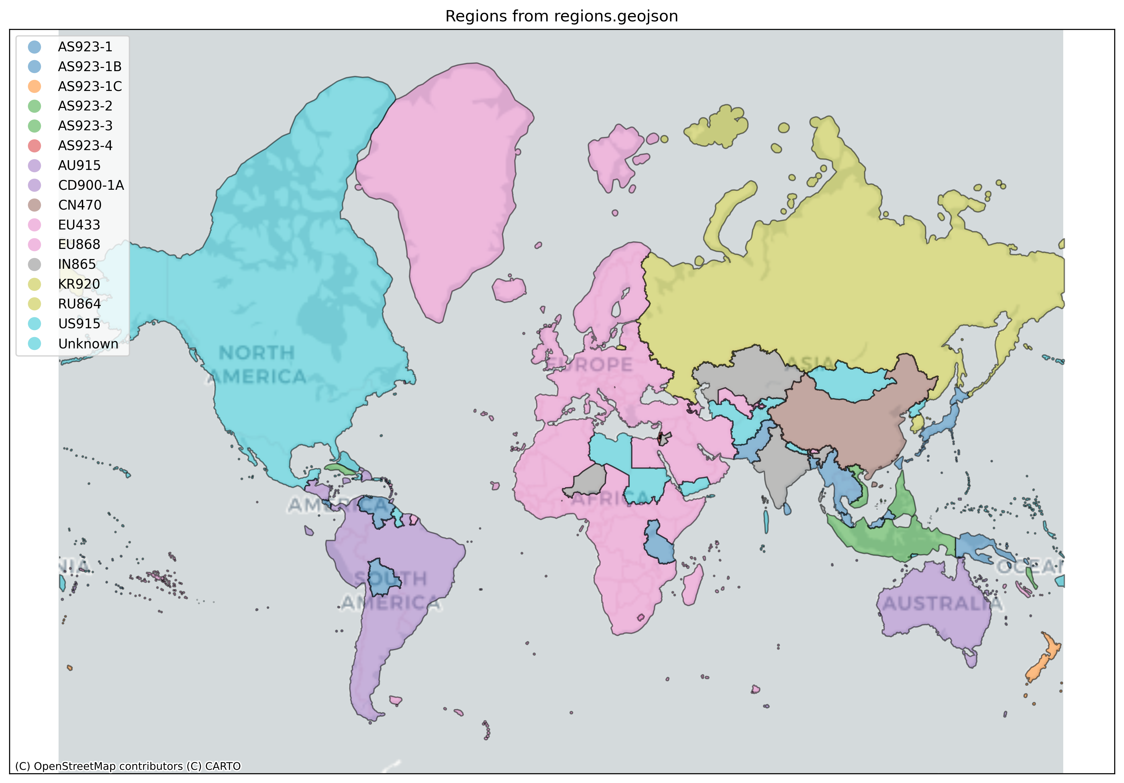 Global LoRaWAN regional coverage from the DEWI Alliance hplans repository
Traditional approaches would require either:
- Using rectangular grid systems (like Maidenhead grid squares) - inadequate for global coverage due to polar distortion and misalignment with regional boundaries
- Storing complete polygon boundary definitions - hundreds of kilobytes of data
- Implementing complex point-in-polygon algorithms - too computationally heavy for an STM32 microcontroller
- Using the full Uber H3 library - over 200KB of flash memory
Our STM32WLE5 microcontroller has limited resources: ~256KB of flash and ~64KB of RAM must accommodate the entire firmware, including the LoRaWAN stack, sensor drivers, and our application logic. We needed a solution that could determine geographic regions using less than 50KB of flash memory and complete lookups in microseconds.
H3Lite: Geospatial Indexing for Embedded Systems
The solution came from adapting Uber’s H3 Hierarchical Geospatial Indexing System—a hexagonal grid system that discretizes the Earth’s surface into cells at multiple resolutions. Like grid squares, H3 provides a compact way to represent location, but with crucial advantages for autonomous region detection. Instead of implementing the full H3 specification, we created H3Lite: a minimalist implementation specifically optimized for our use case.
What is H3?
H3 represents locations on Earth using a hierarchical hexagonal grid. At resolution 0, the Earth is divided into 122 base cells. Each resolution level subdivides each hexagon into 7 child hexagons, creating progressively finer grids. Resolution 3 (our chosen level) divides the Earth into approximately 41,162 cells, each ~100-130km across—perfect for regional boundaries.
The genius of H3 is its encoding: every location on Earth at a given resolution can be represented by a single 64-bit integer. This integer encodes:
- The base cell (0-121)
- The resolution level (0-15)
- The path through the hierarchy to reach that cell
How H3Lite Works: From Location to Region
The transformation from GPS coordinates to a LoRaWAN region happens in three clean steps:
Step 1: Lat/Lng → H3 Hexagon
When the device gets a GPS fix (e.g., 39.74°N, 104.99°W), it converts those coordinates into an H3 index—a unique 64-bit identifier for a hexagonal cell on Earth:
H3Index h3 = latLngToH3(39.74, -104.99, 3);
// Result: 0x832830fffffffff
The H3 index encodes:
- Base Cell (bits 45-52): Which of the 122 root hexagons (0-121)
- Resolution (bits 52-56): Detail level, we use 3 (~100-130km cells)
- Child Path (bits 0-45): Which child hexagon at each subdivision level
Step 2: H3 Index → Lookup Components
We extract just the parts we need for the lookup table:
uint8_t baseCell = 0x42;        // Base cell 66 (from bits 45-52)
uint16_t partialIndex = 0x180;  // First 3 resolution digits (384 in decimal)
These two numbers uniquely identify the hexagon within our resolution 3 grid. Combined, they’re only 3 bytes—much more compact than storing full H3 indexes or polygon coordinates.
Step 3: Lookup → Region ID
Binary search through our sorted table finds the matching entry:
typedef struct {
    uint8_t baseCell;      // 0x42 (base cell 66)
    uint16_t partialIndex; // 0x180 (path through hierarchy)
    RegionId regionId;     // 1 (US915)
} RegionEntry;
The table returns regionId = 1, which maps to “US915”.
The Efficiency Wins:
- Compact Storage: 4 bytes per entry vs 100s of bytes for polygon coordinates
- Fast Lookup: Binary search O(log n) vs point-in-polygon O(vertices)
- Small Memory: ~43.8KB total (10,953 entries) fits easily in flash
- Pre-computed: All complexity happens offline in Python, firmware just does simple lookups
Resolution Trade-offs: The generation script fills regions at a specified resolution (default: 3). Higher resolutions provide more precise boundary definition but require larger lookup tables. The following table compares key characteristics across different resolution levels:
H3 Resolution Comparison Table
| Resolution | Hexagon Edge | Hexagon Diameter | Global Hexagons | Actual Region Entries | Flash Size (4 bytes/entry) | Boundary Precision | Use Case |
|---|---|---|---|---|---|---|---|
| R1 | ~418 km | ~836 km | 842 | ~500-800 (est.) | ~2-3 KB | ±200-400 km | Continent-scale regions only |
| R2 | ~158 km | ~316 km | 5,882 | 1,798 | 7.0 KB | ±80-150 km | Coarse regional coverage |
| R3 | ~60 km | ~120 km | 41,162 | 12,517 | 48.9 KB | ±30-60 km | Balanced (default) |
| R4 | ~23 km | ~46 km | 288,122 | 87,487 | 341.7 KB | ±12-25 km | Precise boundaries (large) |
Key Trade-offs:
- R1-R2: Too coarse for accurate regional boundaries. Small table size but poor precision at edges.
- R3 (default): Optimal balance of ~40-48KB flash usage with ±30-60km boundary accuracy. Perfect for stratospheric applications where transitions happen over hours.
- R4: Excellent precision but prohibitive flash usage (280-400KB) - would consume most available STM32WLE5 memory.
H3’s hierarchical structure provides some automatic compression when all child hexagons within a parent belong to the same region, but the main trade-off remains between edge precision and memory usage. For the Stratosonde, R3 provides sufficient accuracy since:
- The device moves slowly in the stratosphere (10-30 m/s drift)
- Region transitions occur gradually over hours of flight time
- LoRaWAN gateways provide ~20-50km range, making sub-60km precision unnecessary
Regional Coverage Breakdown (Multi-Resolution Analysis)
The following table shows the exact hexagon counts for each region across resolutions R2, R3, and R4, derived from GeoJSON boundary analysis:
| Region | R2 Hexes | R3 Hexes | R4 Hexes | Flash | Typical Countries |
|---|---|---|---|---|---|
| EU868 | 489 | 3,409 | 23,784 | 13,636 bytes | Europe, Middle East, Africa |
| AU915 | 328 | 2,264 | 15,858 | 9,056 bytes | Australia, New Zealand, Pacific |
| US915 | 287 | 2,001 | 13,971 | 8,004 bytes | United States, Canada, South America |
| RU864 | 209 | 1,418 | 9,940 | 5,672 bytes | Russia, Kazakhstan |
| CN470 | 125 | 853 | 6,004 | 3,412 bytes | China |
| AS923-1 | 96 | 684 | 4,780 | 2,736 bytes | Japan, Singapore, Taiwan |
| Unknown | 85 | 643 | 4,471 | 2,572 bytes | N. Korea, Libya, Sudan, Yemen |
| IN865 | 77 | 564 | 3,918 | 2,256 bytes | India |
| AS923-2 | 62 | 434 | 3,063 | 1,736 bytes | Vietnam, Cambodia, Laos |
| AS923-3 | 17 | 114 | 774 | 456 bytes | Philippines |
| EU433 | 9 | 43 | 289 | 172 bytes | Central Asia (limited) |
| AS923-1C | 6 | 36 | 238 | 144 bytes | Indonesia (partial), Timor-Leste |
| AS923-1B | 4 | 33 | 238 | 132 bytes | Brunei, Indonesia (partial) |
| KR920 | 3 | 18 | 142 | 72 bytes | South Korea |
| AS923-4 | 1 | 2 | 13 | 8 bytes | Israel |
| TOTAL | 1,798 | 12,517 | 87,487 | 50,068 bytes | Global Coverage |
| Flash Size | 7.0 KB | 48.9 KB | 341.7 KB |
† Note: EU433 and CN470 are included for completeness but will not be supported in the final hardware, which operates in the 850-950 MHz range. CD900-1A is a test region currently unused in production.
Key Observations:
- Resolution Scaling: R4 requires ~7x more entries than R3, while R2 uses ~7x fewer entries (close to the theoretical 7:1 ratio per H3 subdivision level)
- EU868 Dominates: Europe’s complex geography requires 27% of R3 entries and 27% of R4 entries
- Largest Regions: EU868, AU915, and US915 together account for ~61% of all entries across all resolutions
- Minimal Regions: AS923-4 (Israel) and CD900-1A (Congo) require only 2-4 hexes even at R3
- R4 Impractical: At 341.7 KB, R4 would consume most of the STM32WLE5’s 256KB flash memory
- R3 Optimal: At 48.9 KB, R3 bal ances precision with memory constraints perfectly
Over-Ocean Handling: When flying over oceans where no cell is in the table, H3Lite searches outward in hexagonal rings to find the nearest regions:
NearestRegionsInfo nearest = findNearestRegions(lat, lng, 3);
// Returns: US915 (550km), EU868 (2100km), etc.
The device can then attempt transmission using the closest region’s parameters, maximizing chances of gateway reception.
From hplans to Firmware: The Complete Pipeline
The journey from geographic boundaries to embedded lookup tables involves several carefully orchestrated steps:
Step 1: Defining LoRaWAN Regions
The process begins with GeoJSON files defining each LoRaWAN region’s coverage area. These files come from the DEWI Alliance hplans repository—a community-maintained collection of LoRaWAN regional plan boundaries based on regulatory databases and LoRaWAN Alliance specifications.
Each file contains polygon geometries describing where that region’s frequency plan applies:
{
  "type": "FeatureCollection",
  "features": [{
    "type": "Feature",
    "geometry": {
      "type": "MultiPolygon",
      "coordinates": [...]
    },
    "properties": {
      "region": "US915"
    }
  }]
}
Regions like US915 are straightforward—roughly the United States and territories. Others like AS923 have multiple sub-regions (AS923-1, AS923-2, etc.) with specific country assignments. The challenge is converting these irregular political boundaries into efficient lookup tables.
Step 2: Fill Regions with H3 Hexagons
The generate_lookup_table.py script loads each GeoJSON file and fills the polygon with H3 hexagons at multiple resolutions:
 US915 region filled with H3 hexagons at resolutions 2, 3, and 4. Higher resolutions provide more precise boundary definition but require more table entries.
h3_cells = h3.h3shape_to_cells(polygon, res=3)
# Converts irregular political boundaries into ~11,000 hexagonal cells
Step 3: Extract Components and Build Lookup Table
Each H3 hex is converted into a compact 4-byte entry containing the region ID:
typedef struct {
    uint8_t baseCell;      // Which base hex (0-121)
    uint16_t partialIndex; // Path through subdivisions
    RegionId regionId;     // Which region (1-16)
} RegionEntry;  // 4 bytes total
The table is sorted for fast binary search: ~10,953 entries × 4 bytes = ~43.8KB.
Step 4: Firmware Lookup
In the firmware, GPS coordinates are converted to a region in one function call:
RegionId region = latLngToRegion(lat, lng);

if (region >= 1 && region <= 15) {
    // Valid LoRaWAN region - configure and transmit
    LoRaWAN_SetRegion(region);
}
else if (region == 16) {
    // Unknown/prohibited - block transmission
    LoRaWAN_DisableTransmission();
}
else {  // region == 0
    // Ocean - try nearest regions
    NearestRegionsInfo nearest = findNearestRegions(lat, lng, 3);
    // Attempt transmission to nearest valid regions
}
Three distinct scenarios:
The H3Lite system distinguishes between three distinct geographic scenarios, each requiring different behavior:
1. Valid LoRaWAN Region (IDs 1-15)
When latLngToRegion() returns a valid region ID (1-15), the device has found itself within an established LoRaWAN region:
RegionId region = latLngToRegion(lat, lng);
if (region >= REGION_US915 && region <= REGION_CD900_1A) {
    // Valid region - configure and transmit
    LoRaWAN_SetRegion(region);
    LoRaWAN_Transmit(payload);
}
2. Unknown/Prohibited Region (ID 16 - in lookup table) The Unknown region explicitly marks areas where LoRaWAN transmission is prohibited or where no regulatory framework exists. This includes countries like North Korea, Libya, Sudan, Yemen, Nepal, Mongolia, and various Central Asian states. When the device detects the Unknown region, it blocks all radio transmission:
RegionId region = latLngToRegion(lat, lng);
if (region == REGION_UNKNOWN) {
    // Explicitly prohibited area - do not transmit
    LOG("Entered prohibited transmission area");
    LoRaWAN_DisableTransmission();
    return;
}
This differs from simply not finding a region—the Unknown region is actively present in the lookup table, marking specific geographic areas where the device must not transmit.
3. Ocean/No Coverage (no match in lookup table)
When flying over oceans or remote areas where no H3 cell is in the lookup table, latLngToRegion() returns 0 because no match was found. In this case, the device attempts to communicate with nearby regions:
RegionId region = latLngToRegion(lat, lng);
if (region == 0) {
    // No region found - try nearest regions
    NearestRegionsInfo nearest = findNearestRegions(lat, lng, 3);

    if (nearest.numRegions > 0) {
        // Attempt transmission to nearest region(s)
        for (int i = 0; i < nearest.numRegions; i++) {
            RegionId nearRegion = nearest.regions[i].regionId;

            // Skip Unknown region even if it's nearest
            if (nearRegion != REGION_UNKNOWN) {
                double distance = nearest.regions[i].distanceKm;
                LOG("Trying region %s at ~%.0f km",
                    getRegionName(nearRegion), distance);

                LoRaWAN_SetRegion(nearRegion);
                LoRaWAN_Transmit(payload);
            }
        }
    }
}
The key distinction: Unknown region = actively prohibited (region ID 16 in table), while ocean = no region defined (not found in table, returns 0). This makes them easily distinguishable:
region == 0: No cell found in table → try nearest regionsregion == 16: Unknown region found → block transmissionregion >= 1 && region <= 15: Valid LoRaWAN region → configure and transmit
This three-way distinction ensures the Stratosonde respects regulatory boundaries while maximizing communication opportunities over international waters.
Performance Characteristics
The implementation achieves our design goals:
Memory Usage
- Core H3Lite code: ~2-4KB flash
- Lookup tables: ~43.8KB flash (10,953 entries × 4 bytes)
- Region names: ~200 bytes flash
- Runtime RAM: <100 bytes
- Total: ~46KB flash, <1KB RAM
Timing Performance (STM32WLE5 @ 48MHz - measured)
latLngToRegion()direct lookup: 2ms- Ring 1 search: 4ms (~65km radius)
- Ring 2 search: 8ms (~130km radius)
- Ring 3 search: 14ms (~195km radius)
- Ring 4 search: 22ms (~260km radius)
- Ring 5 search: 32ms (~325km radius)
- Ring 6 search: 43ms (~390km radius)
Region detection is effectively instantaneous compared to GPS acquisition (1-60 seconds) and LoRaWAN transmission (several seconds). Direct lookups complete in just 2ms, while even the most exhaustive 6-ring offshore search completes in under 50ms.
Accuracy At resolution 3 (~100-130km cell size), boundary accuracy is typically within 50-100km of actual regulatory boundaries. This is more than adequate for stratospheric applications where:
- The device moves relatively slowly (10-30 m/s drift)
- Region transitions are gradual (hours of flight time)
- LoRaWAN gateways have ~20-50km range
Real-World Operation
Consider a typical Stratosonde flight:
T+0 hours: Launch from Colorado
GPS: 39.7392°N, 104.9903°W
H3 Index: 0x832830fffffffff
Region: US915
Action: Configure for 902-928 MHz, SF7-SF10
T+6 hours: Eastern Colorado Still over US915 territory, continues normal operation.
T+24 hours: Over Atlantic, 500km east of Newfoundland
GPS: 47.5°N, 48.2°W
H3 Index: 0x832194fffffffff
Region: Not found (over ocean)
Nearest: US915 (550km W), EU868 (2100km E)
Action: Attempt transmission to US915
T+36 hours: Approaching Ireland
GPS: 52.8°N, 15.4°W
H3 Index: 0x831c4afffffffff
Region: EU868
Action: Switch to 863-870 MHz parameters
The transition is seamless and automatic, requiring no ground intervention.
Regional H3 Coverage Visualizations
The following images show how H3 hexagons at different resolutions cover each LoRaWAN region. Click any image to view the full-size version.
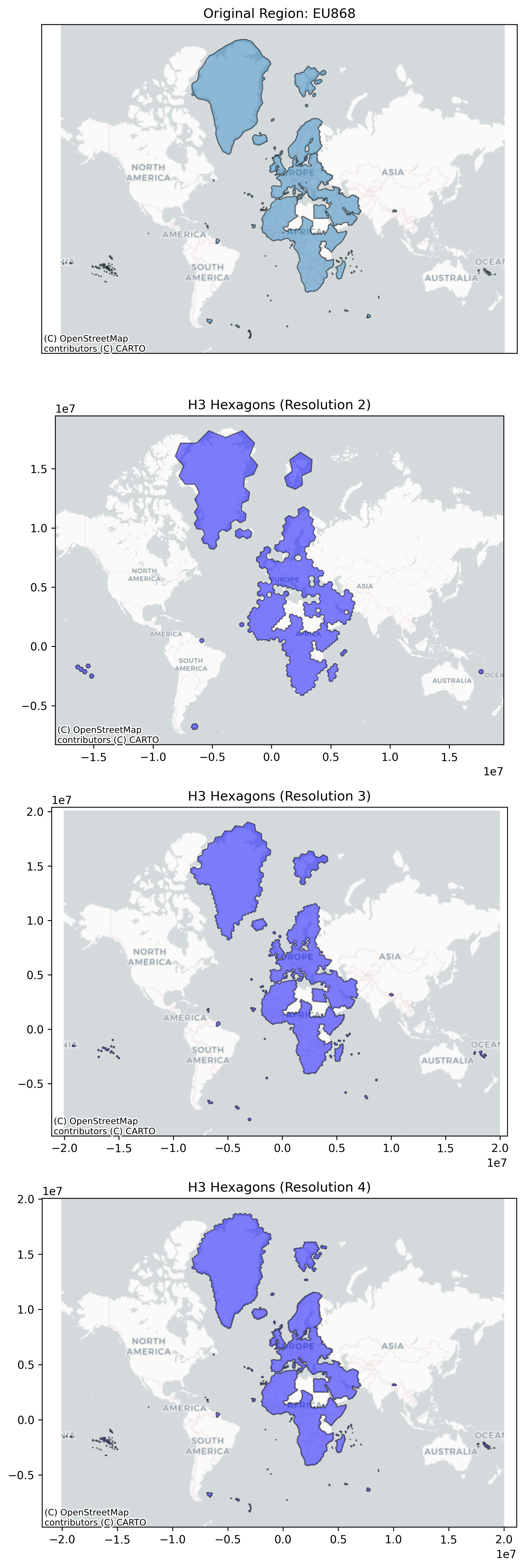
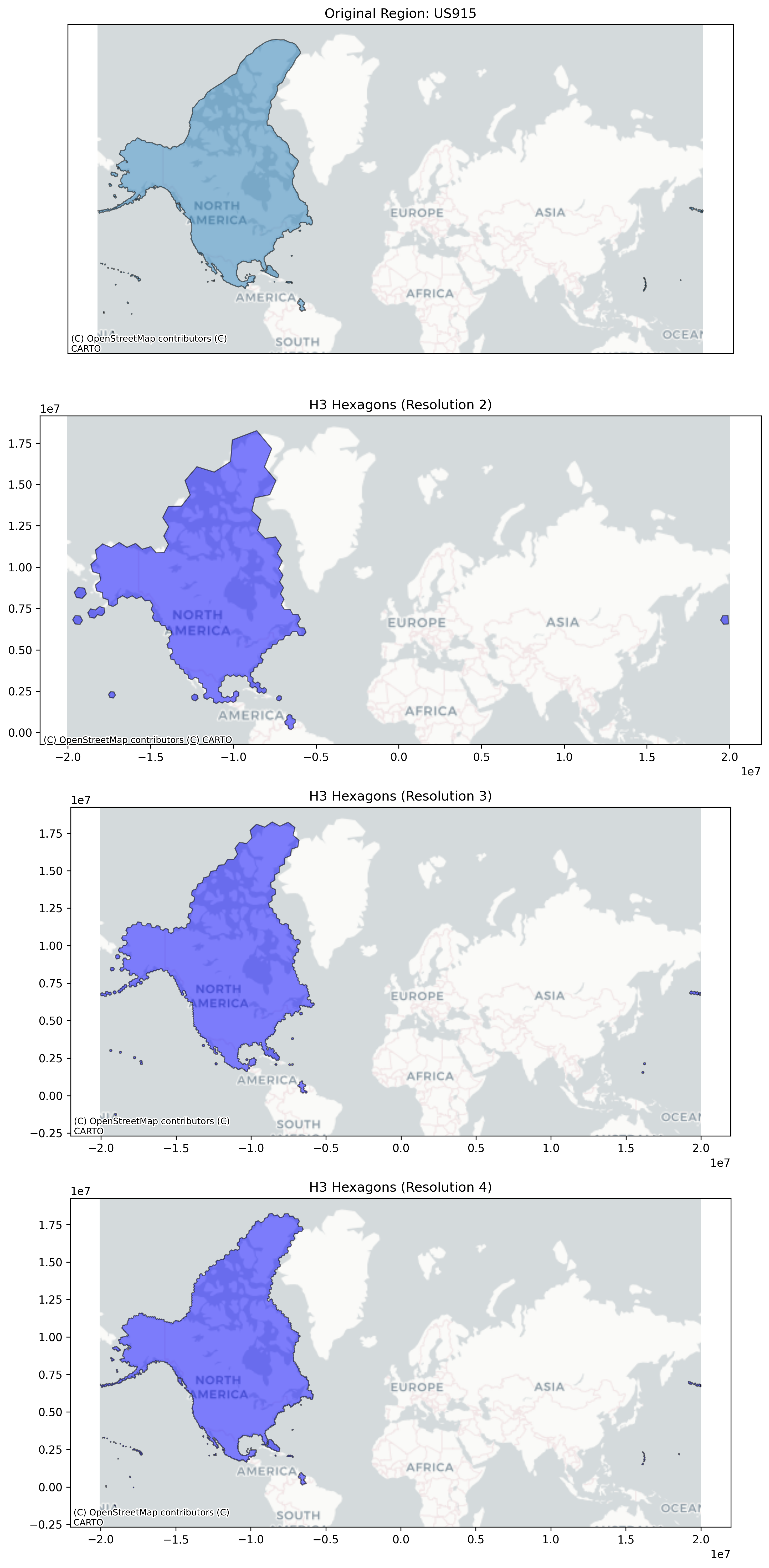
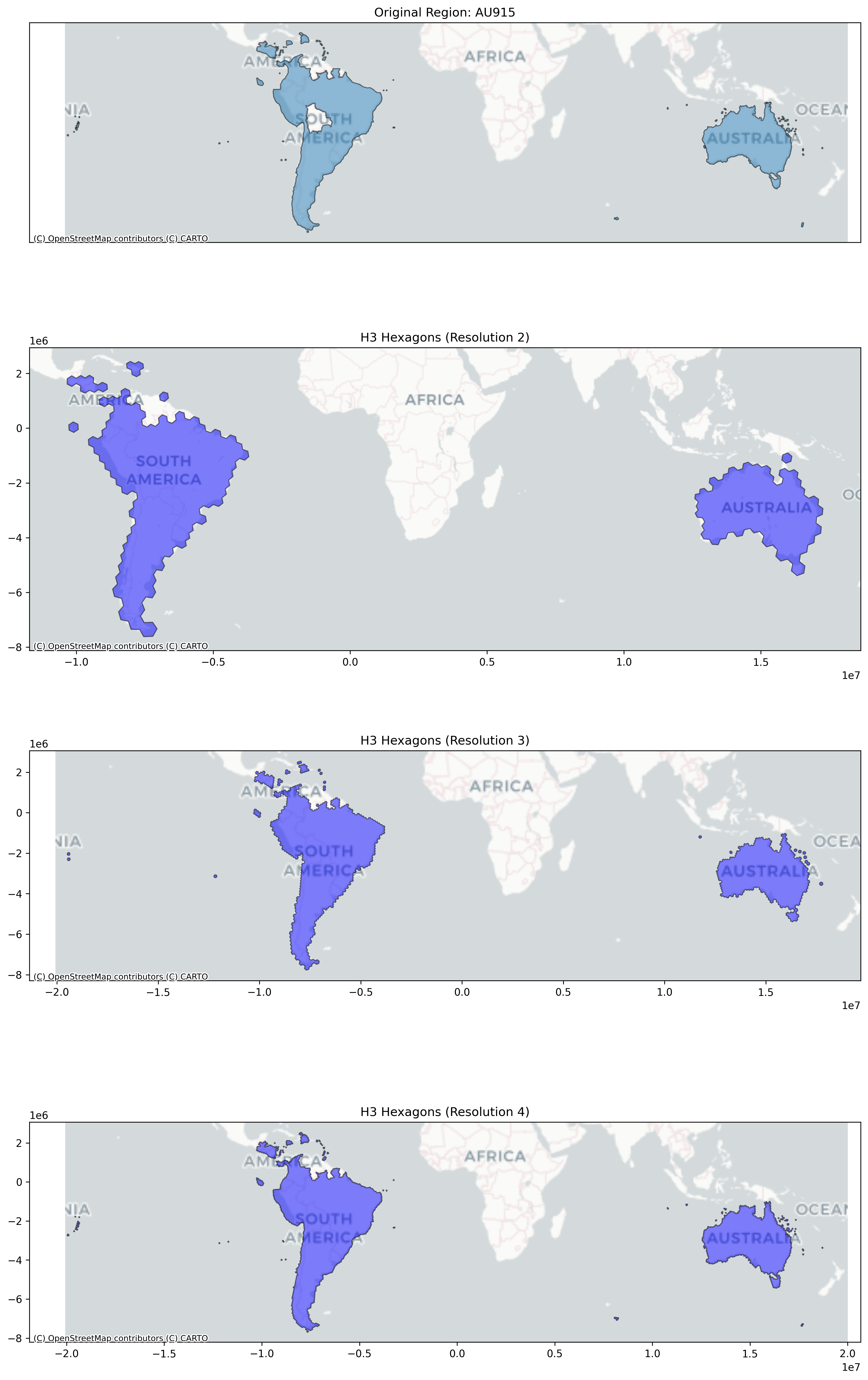
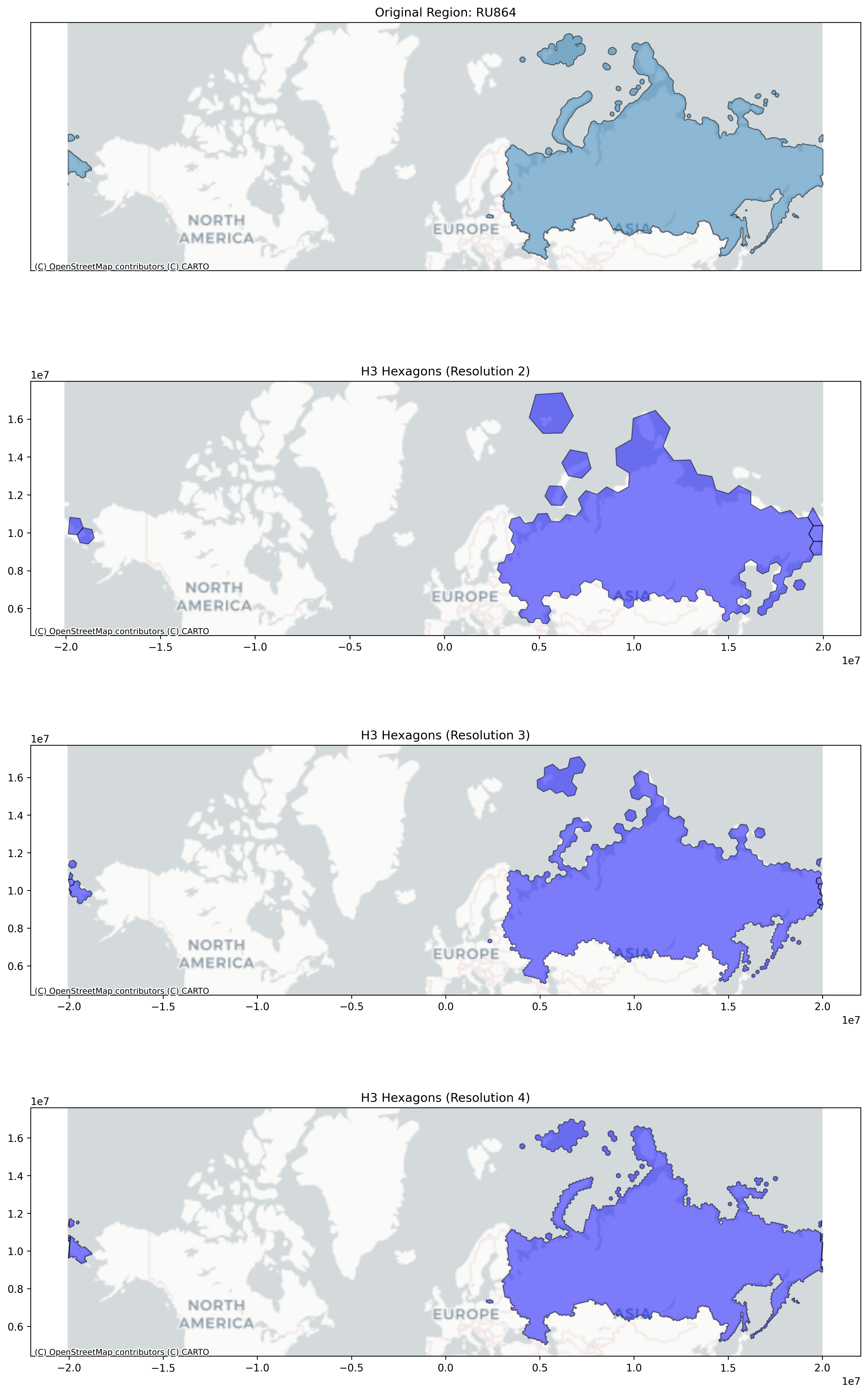
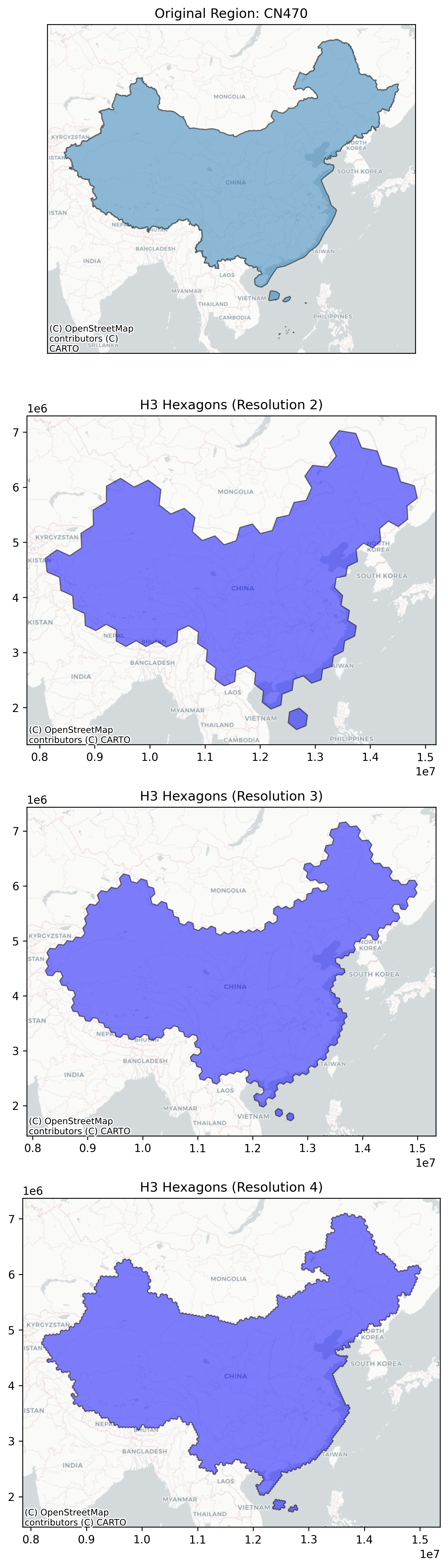
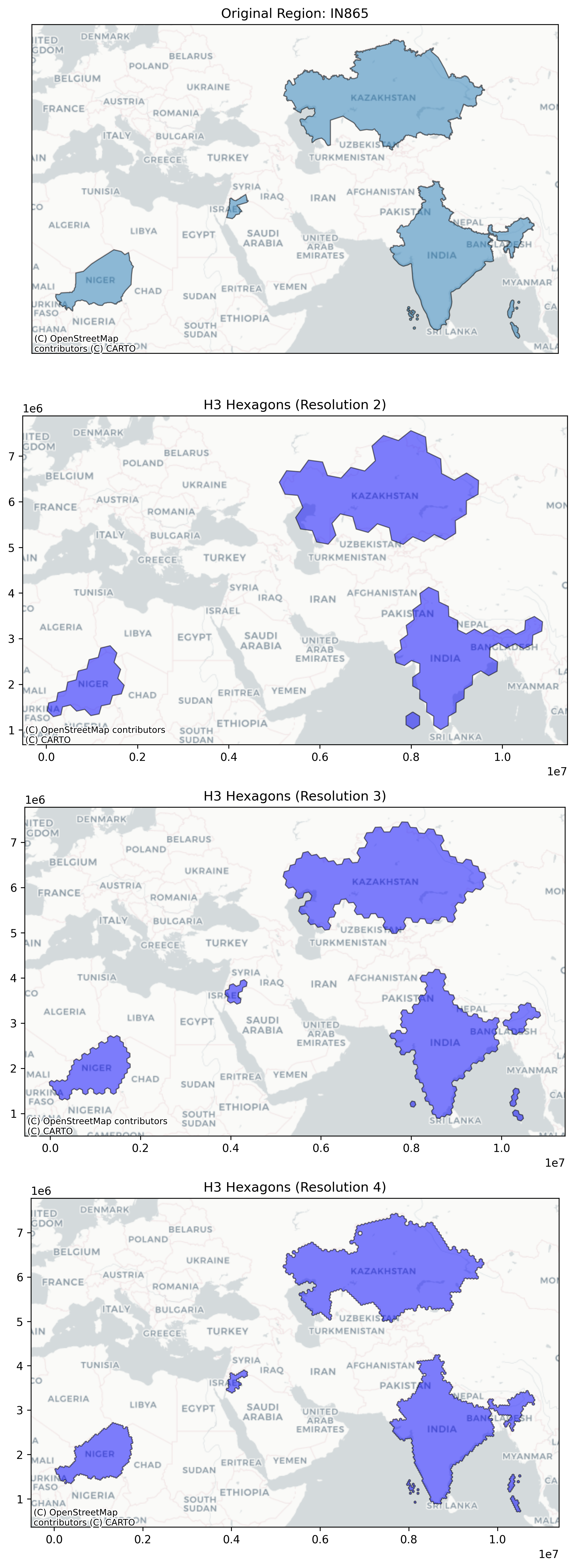
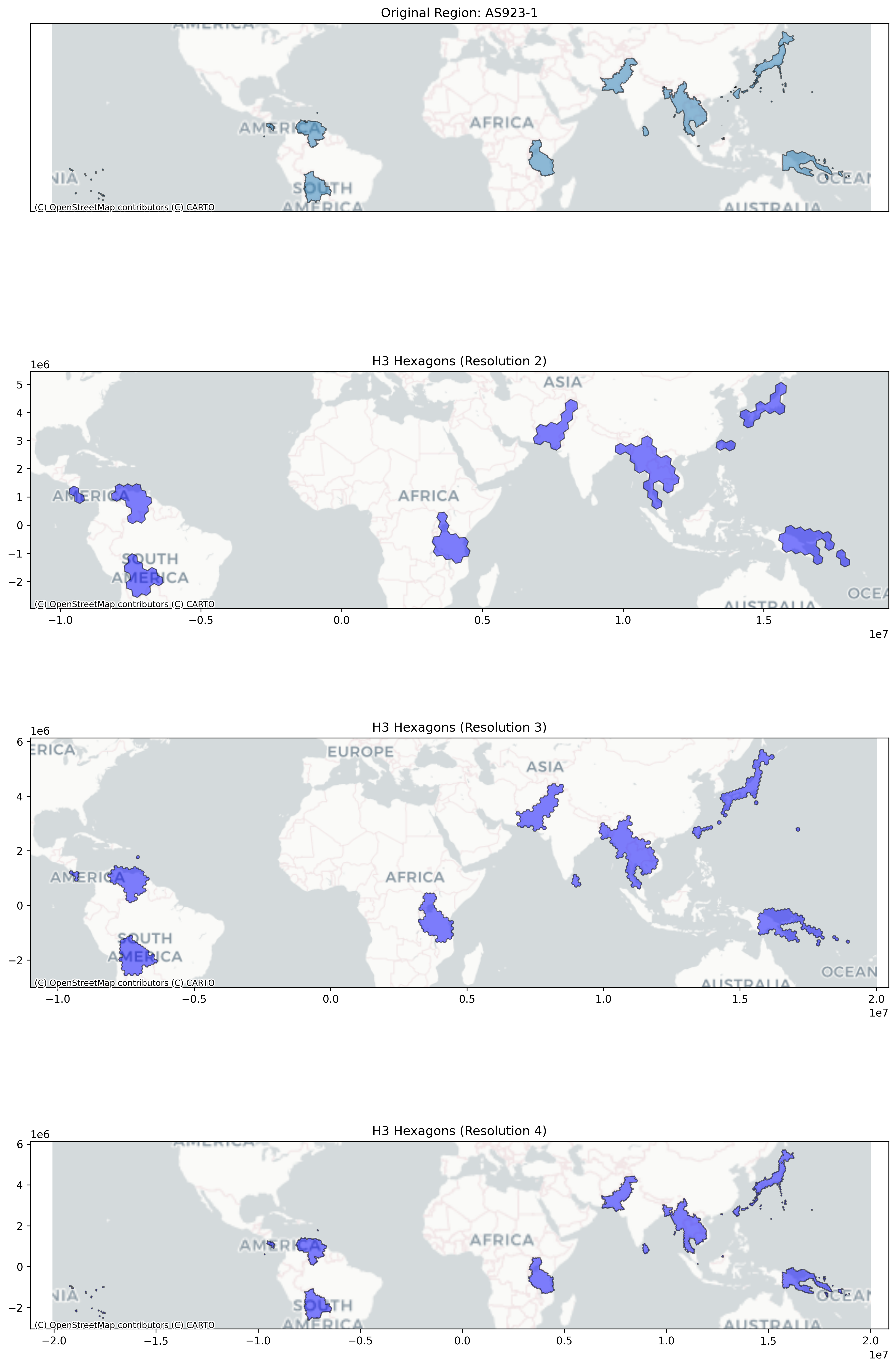
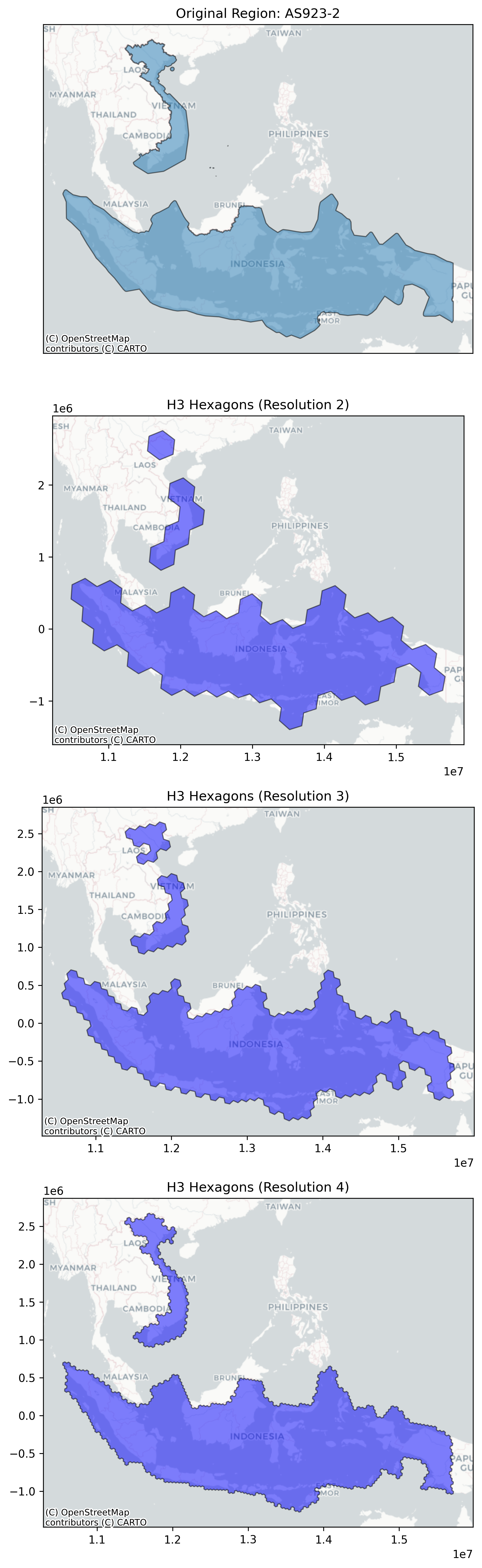
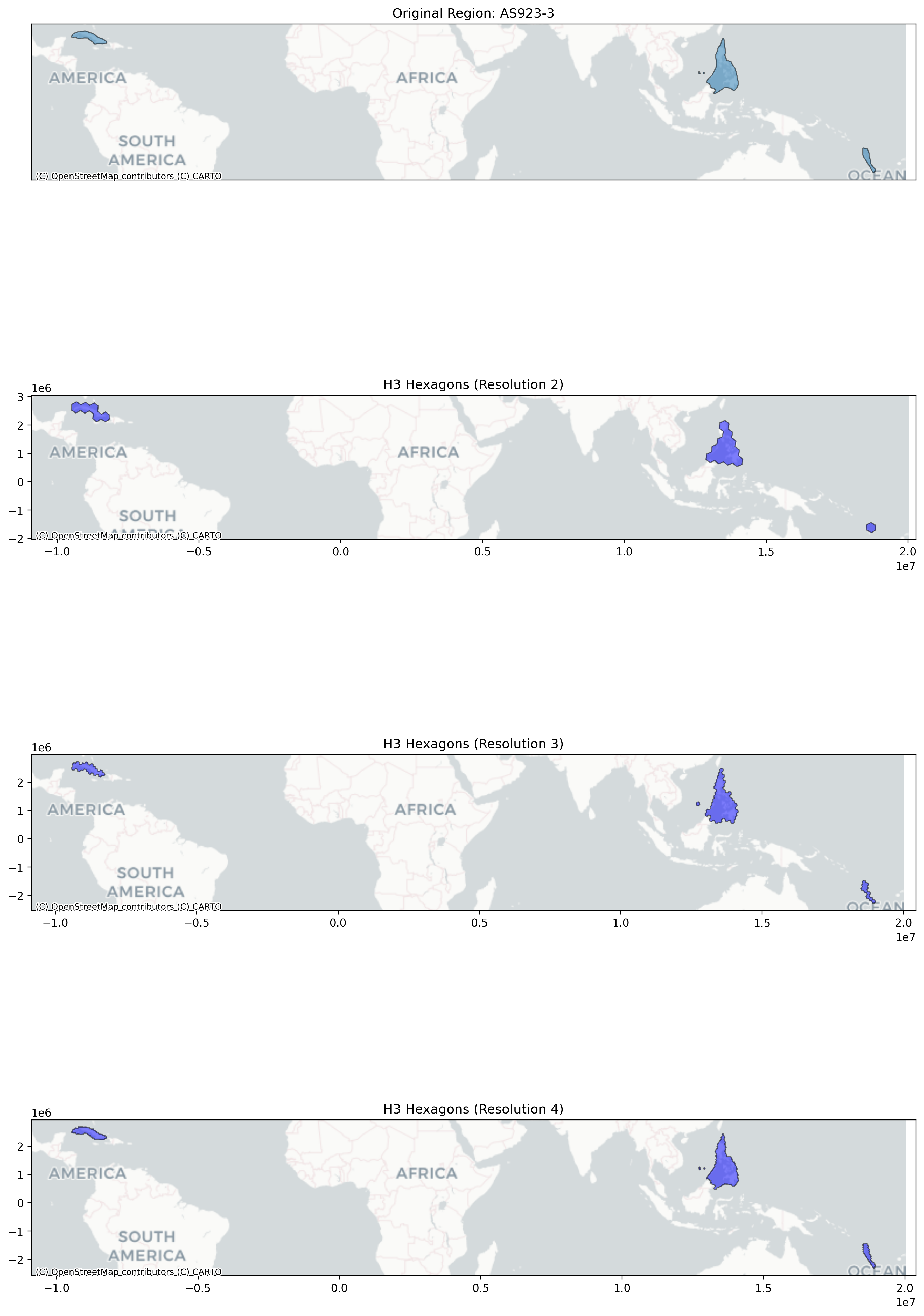
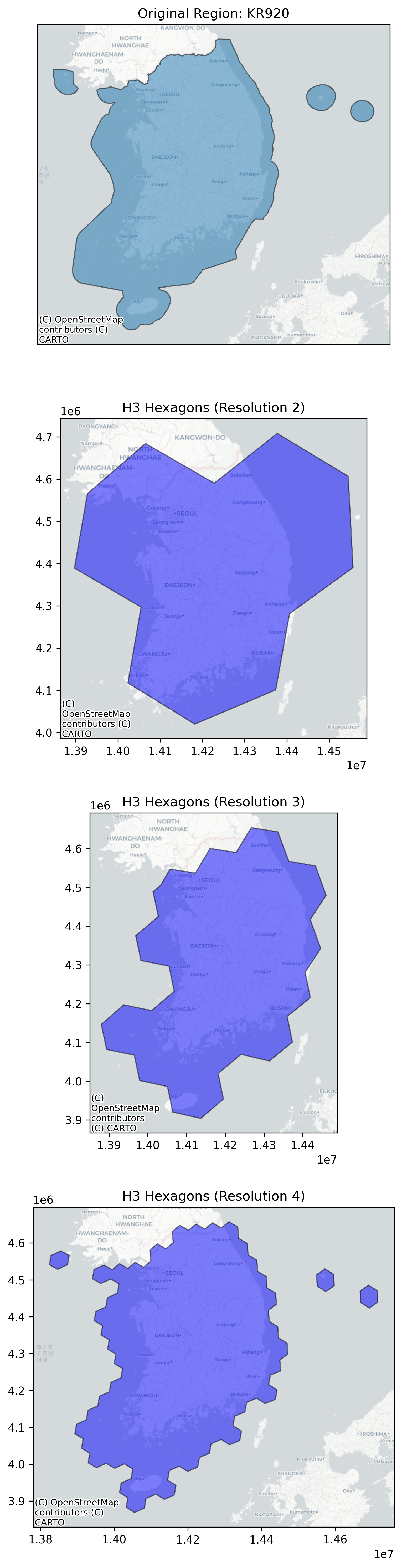
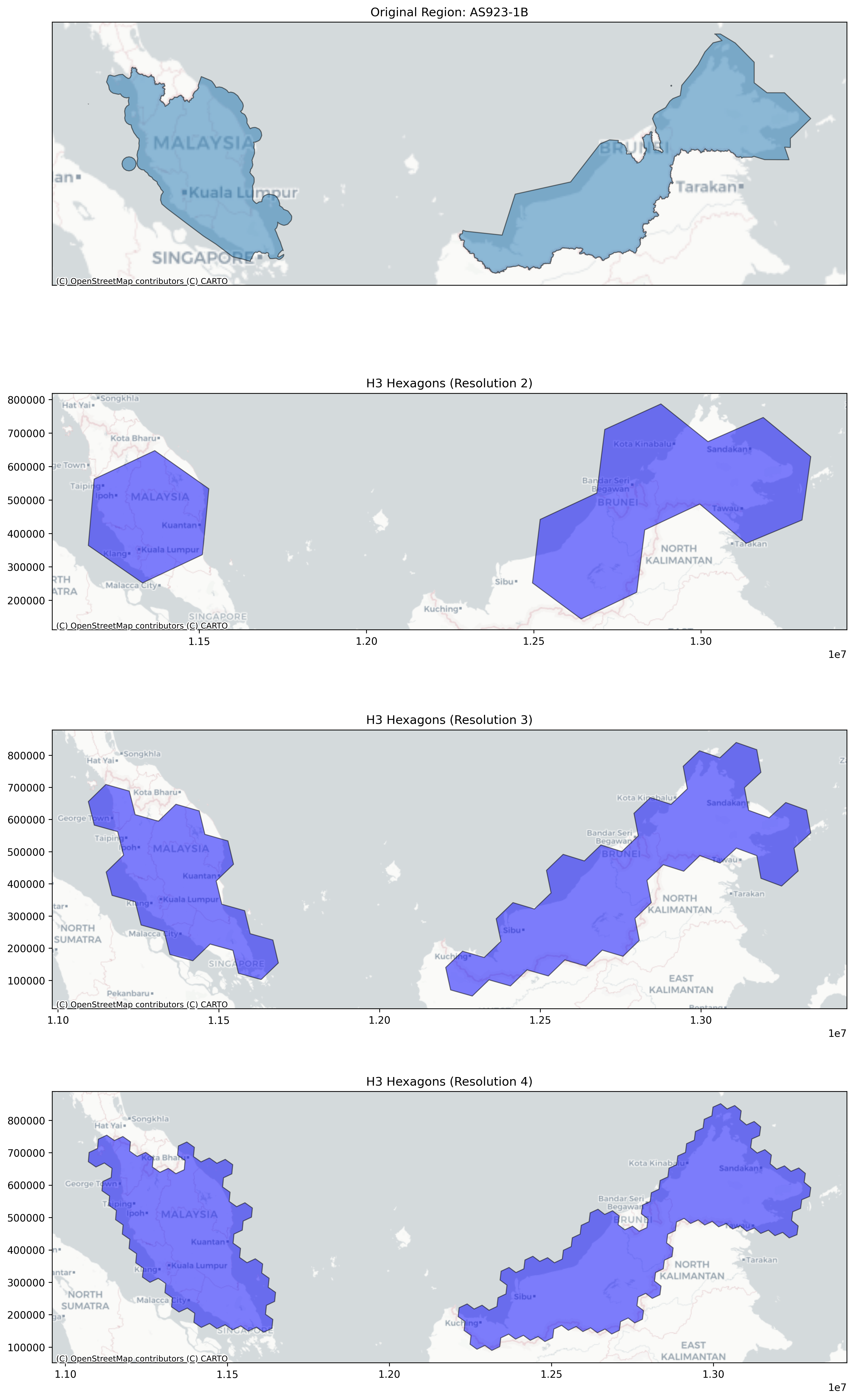
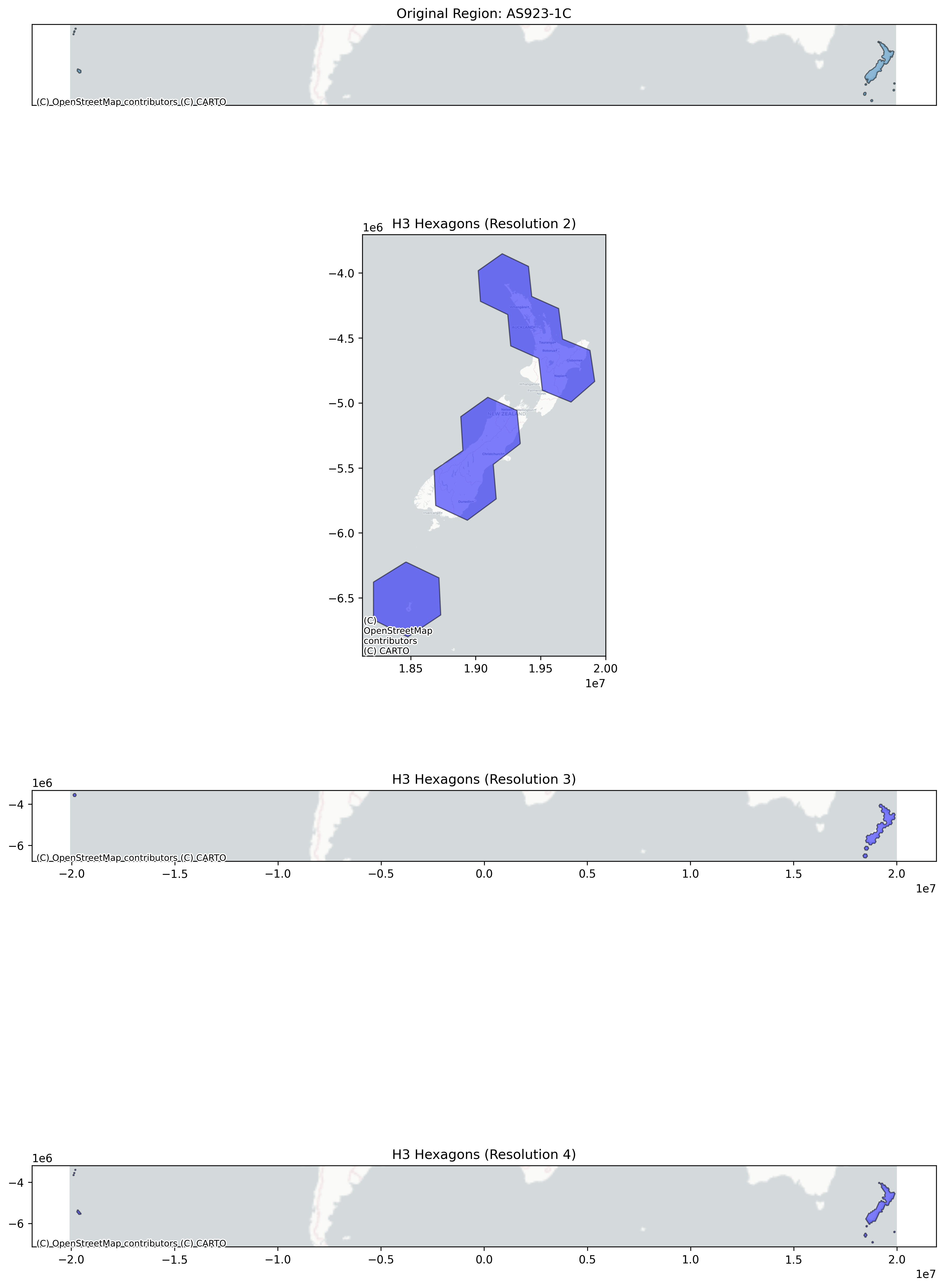
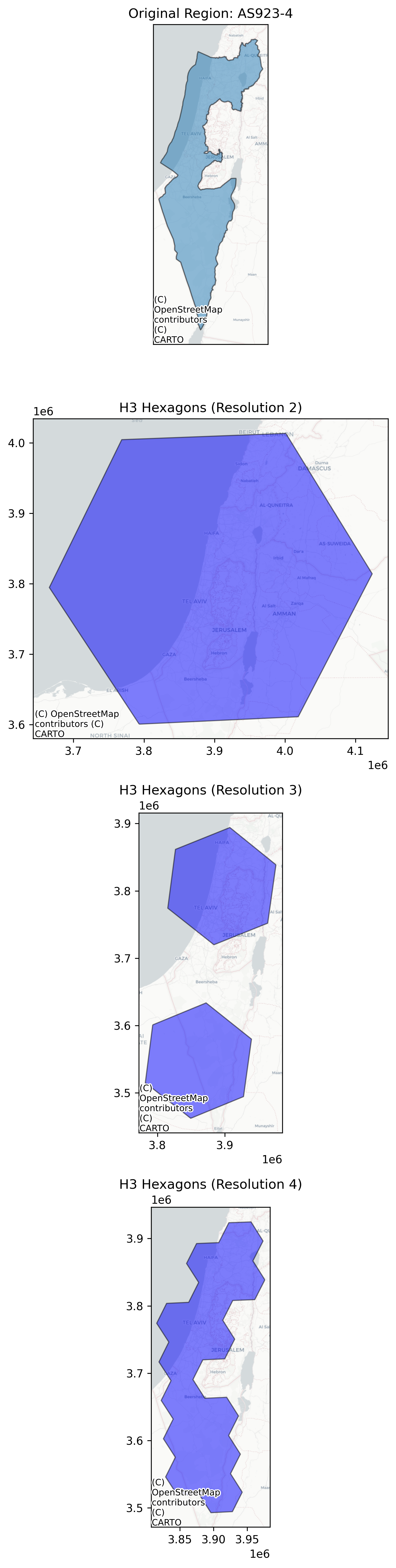
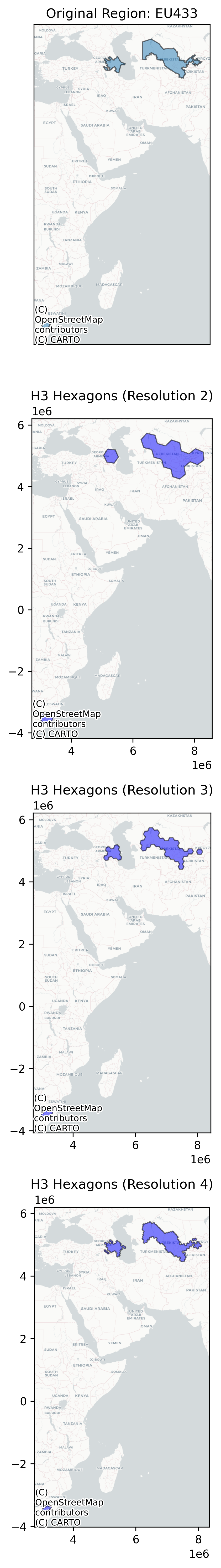
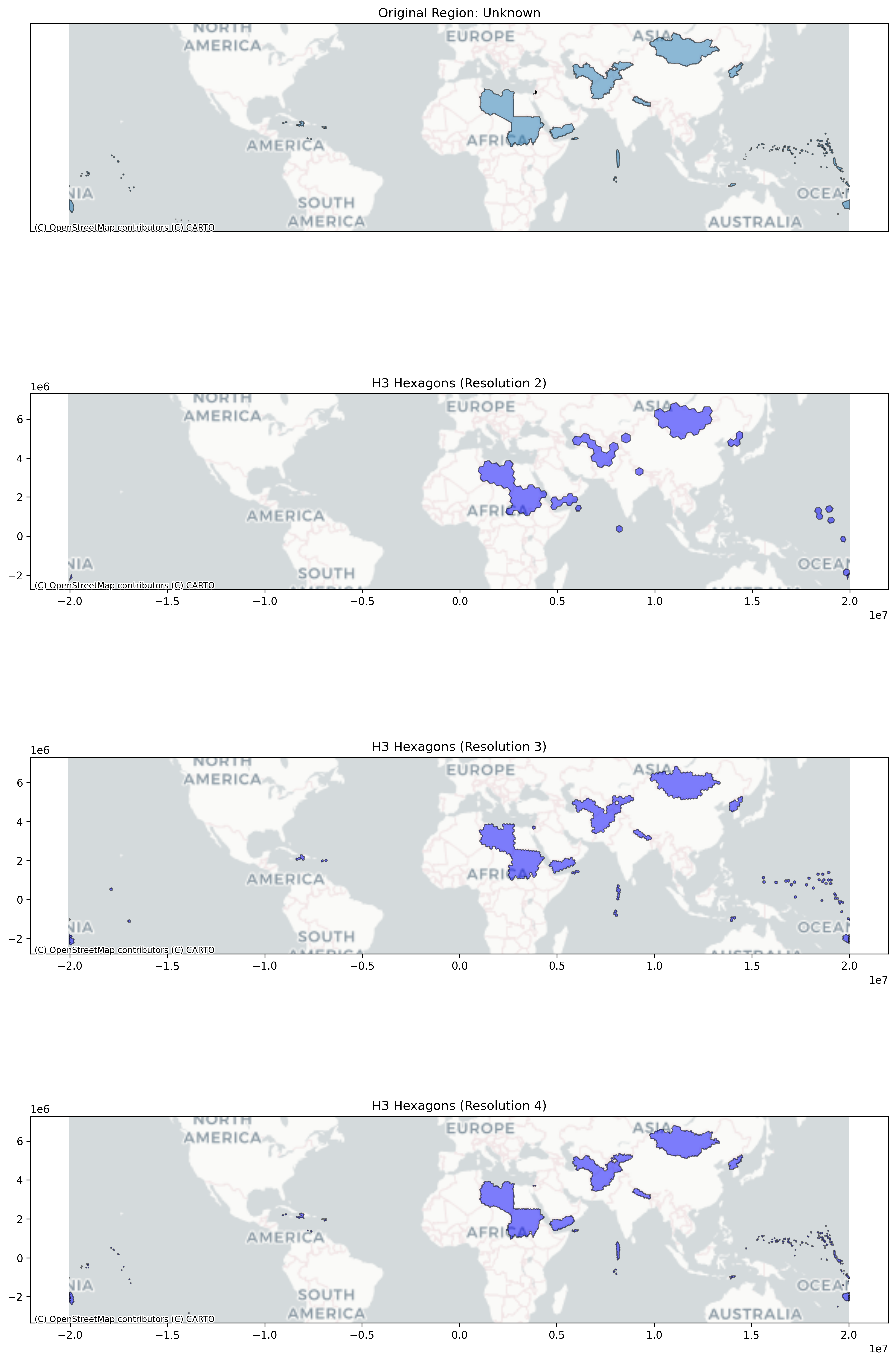
Each visualization shows the region filled with H3 hexagons at resolutions 2, 3, and 4, demonstrating how higher resolutions provide more precise boundary definition.
Interactive Visualization Tool
Want to explore how H3 hexagons cover different LoRaWAN regions? We’ve created an interactive 3D visualization tool using CesiumJS that lets you:
- View LoRaWAN regional boundaries on a 3D globe
- Generate H3 cells at different resolutions (R0-R6)
- Compare resolution trade-offs visually
- Understand how the Stratosonde detects regions

Launch the Interactive Viewer →
The tool provides real-time visualization of how H3 hexagons fill region boundaries, making it easy to understand the firmware’s region detection behavior and explore different resolution trade-offs.
Lessons Learned and Future Directions
Developing H3Lite taught us several valuable lessons:
1. Pre-computation is Power By moving complexity from runtime to build time, we achieved a 50x reduction in flash usage compared to runtime spatial algorithms. The Python table generation script takes minutes to run but enables microsecond lookups.
2. Multi-Resolution is Elegant Using hierarchical resolutions reduced table size while maintaining accuracy. Resolution 1 provides broad coverage, resolution 3 provides precision if needed.
3. Binary Search is Underrated Modern embedded developers often reach for hash tables or trees. For static datasets, sorted arrays with binary search are hard to beat: zero RAM overhead, excellent cache performance, and predictable timing.
4. Embedded Systems Need Specialized Solutions The full H3 library is excellent for server applications but inappropriate for microcontrollers. Creating a focused, optimized implementation was essential.
Conclusion
H3Lite demonstrates that sophisticated geospatial algorithms can run on resource-constrained embedded systems with careful design. By combining Uber’s elegant H3 system with embedded-specific optimizations, we created a solution that:
- Enables truly autonomous operation across continents
- Fits in available flash memory
- Completes lookups in microseconds
- Handles complex real-world scenarios (oceans, boundaries, restricted areas)
The Stratosonde can now fly anywhere on Earth and automatically configure itself for legal, effective communication—a critical capability for long-duration autonomous atmospheric research.
For embedded developers facing similar challenges, H3Lite is available as open-source software under the Apache 2.0 license. Whether you’re building autonomous drones, wildlife trackers, or mobile IoT devices, the principles and code can help solve your geospatial indexing needs.
The H3Lite library and Stratosonde firmware are available at [github.com/stratosonde/h3lite]
Technical Specifications
| Parameter | Value |
|---|---|
| Target MCU | STM32WLE5JC (ARM Cortex-M4) |
| Flash Usage | 46KB (tables) + 4KB (code) = 50KB |
| RAM Usage | <1KB |
| Lookup Time | 2ms direct, 8ms (2-ring offshore search) |
| Resolution | H3 Resolution 3 (~100-130km cells) |
| Coverage | 16 regions globally (15 LoRaWAN + 1 Unknown) |
| Table Entries | 10,953 entries |
| Accuracy | ±50-100km at region boundaries |
Related Posts:
- H3Lite Hardware Validation: STM32WL Profiling Results - Real hardware timing measurements and profiling data
Supported Regions
- LoRaWAN Regions (15): EU868, US915, CN470, AU915, AS923-1, AS923-1B, AS923-1C, AS923-2, AS923-3, AS923-4, KR920, IN865, RU864, EU433, CD900-1A
- Special Regions (1): Unknown (prohibited transmission areas: North Korea, Libya, Sudan, Yemen, Nepal, Mongolia, Central Asian states)